selig S1223 flow on earth and mars
This is a small project I worked on a while back, since I have some free time on my hands, I wanted to revisit the reports and then try to re-explain (mostly to myself) all the intrinsic details of the wonderful world of CFD. Imagine a Selig S1223 aerofoil slicing through Earth’s cozy air versus Mars’ thin atmosphere. I threw it into ANSYS Fluent, crunched some numbers, and drew some MATLAB plots.
Humanity has big dreams, colonize the red planet, and fly drones or whatnot there. But Martian atmosphere is 1% of Earth’s density, 600 Pa pressure, and gravity is 3.7 m/s². Flying there will be like trying to swim in a kiddie pool. I picked the S1223 because it’s a low Re (reynolds number), high lift champ. 12.1% thickness at 19.8% chord, 8.1% camber at 49%, you can refer to the details of this aerofoil here. This aerofoil is perfect for squeezing lift out of nothing.
Geometry Setup
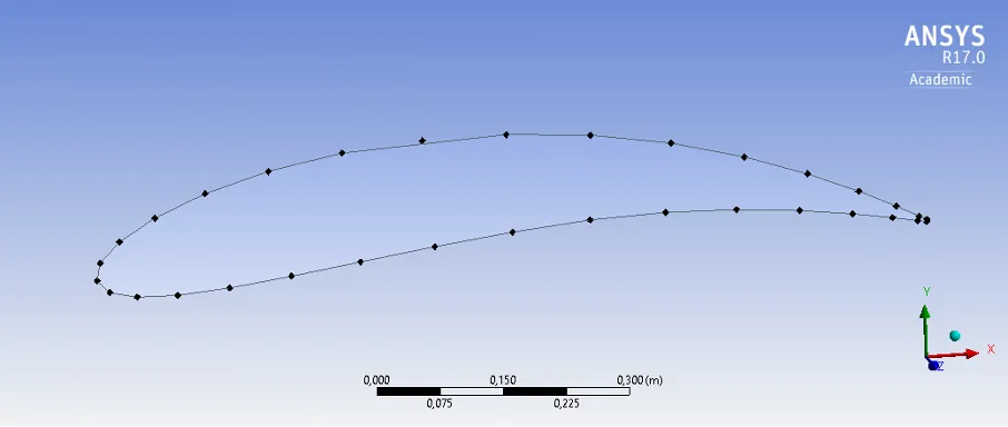
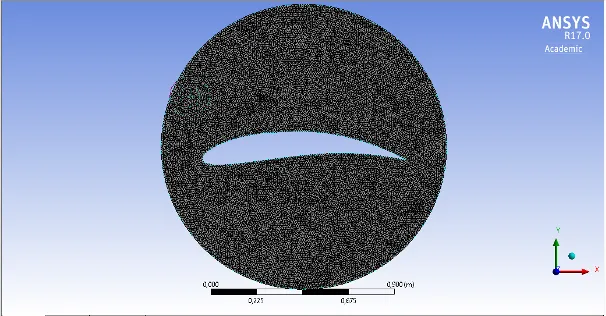
I pulled the S1223’s properties from NACA (2D points that make the aerofoil on a cartersian space). In ANSYS Design Modeler, I imported those points, connected them with splines to get the aerofoil, nose at (0,0). Then, a domain was constructed around the aerofoil with a diameter of 10 chord length. Why 10? Well, I figured that’s far enough to avoid boundary interference (and also in line with common CFD practices). The domain size , where c = 1mc, for simplicity, gives a radius of 10 m. Then, I subtracted the aerofoil shape using a Boolean op, leaving a hollow wing-shaped cutout.
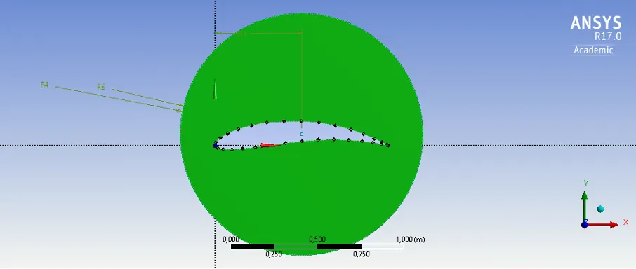
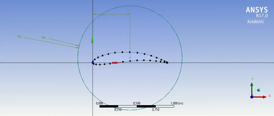
Then, I added a semicircle upstream (radius 5 chords) to define the inlet, connected it to the outer circle with straight lines, and split the domain into two zones: a fluid region and a rotating region for transient cases later. The final geometry is shown below.
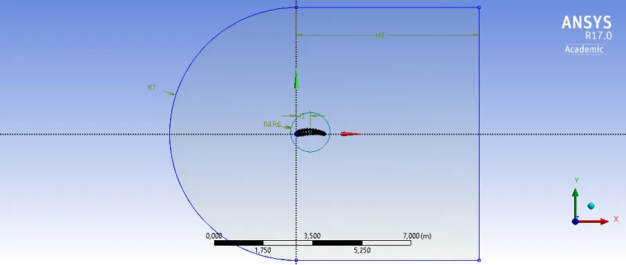
It’s all 2D, because 3D would’ve tanked my pc, and frankly, I didn’t have the computational power. But 2D captures the core physics, and I’m not trying to simulate an Airbus.
Meshing
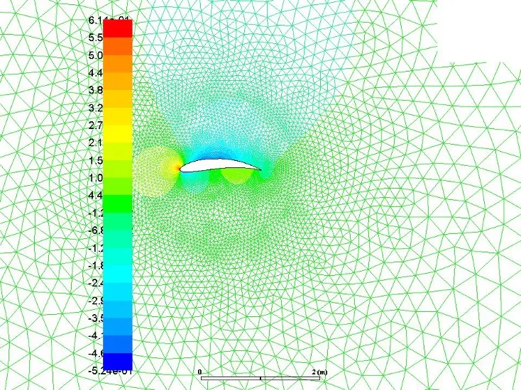
I went with a triangular mesh. Around the aerofoil, I set an element size of 0.01 m (tight for detail), easing to 0.02 m near the inner circle, and 1.0 m max size out in the far field.
After hitting “Generate Mesh,” I got the following figure.
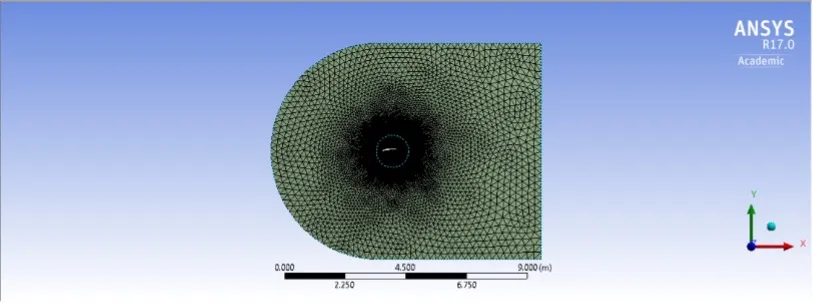
The stats? Orthogonal quality of 0.97 and skewness of 0.0356. That’s pretty good for the analysis that I would need to do.
Why does this matter? The Navier-Stokes equations I am trying to solve are partial differential equations (PDEs). Discretize them on a garbage grid, and you’re begging for numerical diffusion or worse, Divergence!
The discretization error scales with for second order schemes, so finer grids near the aerofoil are crucial. The mesh quality metrics, which is orthogonal quality (Q) , where is the angle between face normals and element edges, and skewness , ensure the solver doesn’t choke.
Fluent Setup
I fired up Fluent and set up a transient, pressure based solver. Transient case would be ideal for me to look at rotating cases later. For the momentum equation, I picked a second-order upwind scheme because the Peclet number () is way above 2 here, i.e., convection dominates diffusion, and first order schemes will smear the solution like a bad watercolor. Second order adds a correction term, sharpening the velocity and pressure fields. The scheme is:
where is the variable (velocity, pressure), ( C ) is the cell center, and ( f ) is the face. It’s a Taylor expansion, basically, and it keeps the physics crisp.
Coupling pressure and velocity was quite an ordeal. I started with SIMPLE, but the residuals wobbled. Tried SIMPLEC and PISO, same outcome. After some research, I chose the COUPLED algorithm. It solves pressure and velocity together in one matrix, no staggered nonsense. For transient flows with big time steps (0.01 s here), it’s a lifesaver. Convergence? Silky smooth after that switch.
Boundary conditions were 10 m/s inlet velocity (x-direction), zero gauge pressure at the outlet, and no slip walls on the aerofoil. Earth’s air is 1.225 kg/m³, 1.81e-5 Pa·s viscosity; Mars is 0.015 kg/m³, 1.42e-5 Pa·s. Reynolds number () with a 1 m chord? ~670,000 on Earth, ~10,500 on Mars. Low Re flow on Mars is a whole different game, more laminar, less turbulent. Mach number? Mars at 10 m/s is ~0.03, so incompressible is fair. The core equations are the incompressible Navier-Stokes:
- Continuity:
- Momentum:
Lift and drag come from surface integrals:
- Lift:
- Drag:
Here, is the angle of attack (AoA), ( p ) is pressure, and is shear stress. Coefficients normalize by dynamic pressure: , .
Earth vs. Mars
I ran three conditions:
- Zero AoA
- Non-zero AoA
- Rotating aerofoil.
Here’s the breakdown, with figures to follow.
Zero AoA
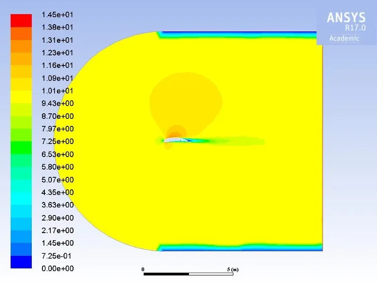
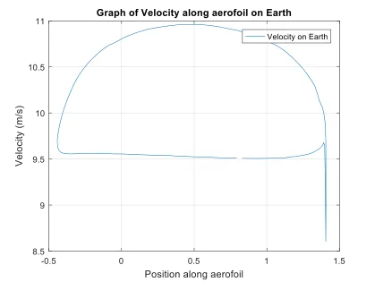
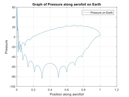
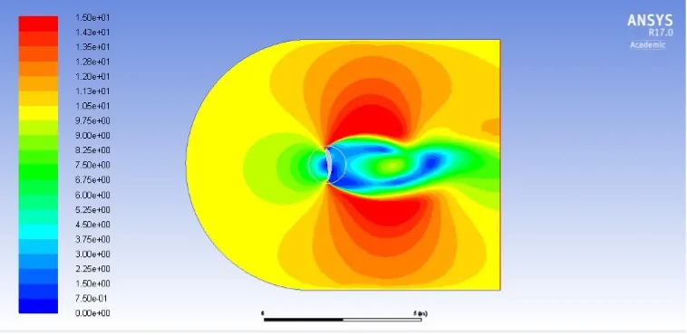
- Earth: Velocity contours show a peak of 11 m/s over the top, Bernoulli’s principle in action with faster flow, lower pressure. The pressure plot dips to -20 Pa (gauge) on the upper surface, driving 55 N of lift. Drag’s ~5 N. , .
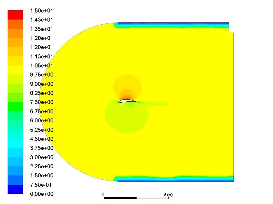
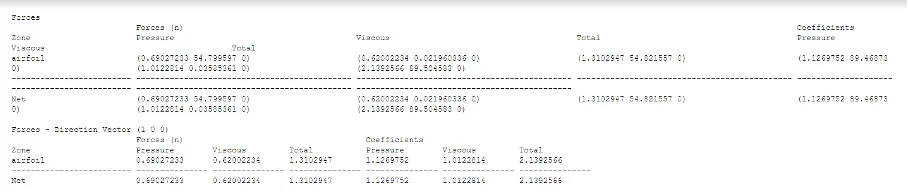
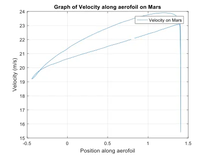
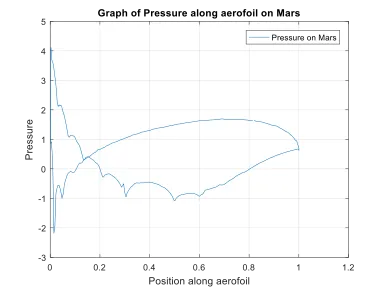
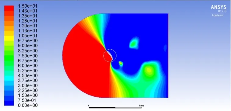
- Mars: Velocity is higher at 24 m/s, less resistance in that thin air. Pressure barely nudges 2 Pa, netting 1 N of lift. , . Martian low density is prevalent here.
Why the gap? Lift scales with , and Martian is 80x smaller. Even with higher velocity, it’s a losing battle. Plus, a 1/3 of Earth's gravity means you need less lift to hover, but 1 N won't cut it.
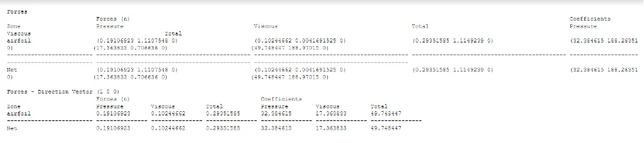
Non-Zero AoA
- Earth: Increasing the AoA to 5°, and velocity hits 12 m/s, with pressure dropping further, lift jumps to ~70 N. The pressure gradient steepens, and you can feel the wing wanting to soar.
- Mars: Velocity pushes 25 m/s, pressure creeps to 3 Pa, and lift nudges up to 1.5 N. Better, but still anemic.
The AoA boost follows the lift equation -> . More angle, more perpendicular pressure force.
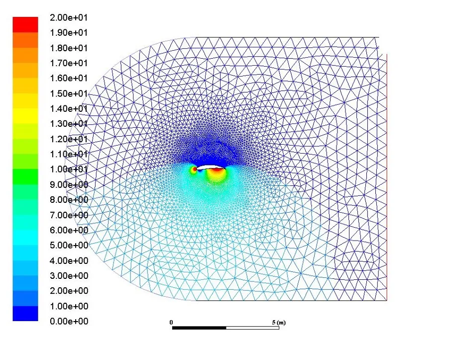
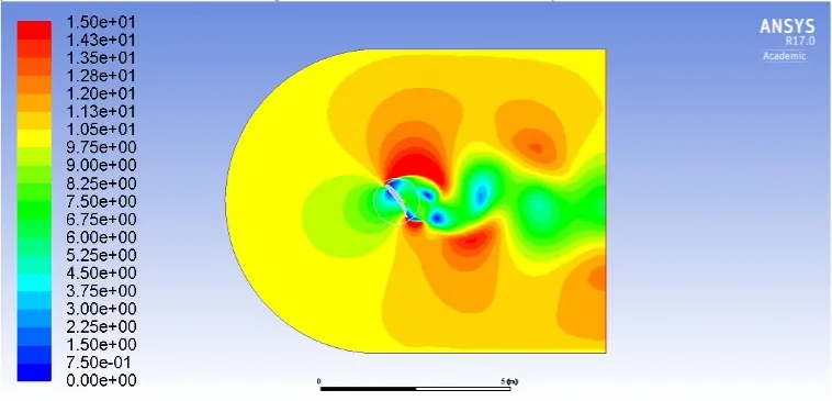
Rotating Case
For kicks, I spun the aerofoil at 10 rad/s in a transient sim. Earth’s velocity shows vortex shedding and wild eddies trailing off. Pressure swings hard, peaking at 50 Pa. Mars is tamer with less density but still sheds vortices. Lift oscillates, Earth averages ~60 N, Mars ~1.2 N.
Plots
Earth’s pressure plot shows a sharp -20 Pa dip at 20% chord, peak lift zone. Mars is flatter, maxing at 2 Pa. Velocity plots for Earth and Mars mirror this. Earth peaks at 11 m/s, Mars at 24 m/s. These are 1D slices, but they show the density variations clearly.
Reflections
The S1223 is quite f]good for low Re lift on Mars, but the thin air is a brutal limiter. Earth’s 55 N vs. Martian 1 N is a huge difference. We will need bigger wings, higher speeds, or maybe active flow control.
The rotating case was a surprise, unsteady flow could be a cheat code for Martian drones. If I redid this, I’d sweep AoA from -10° to 20°, refine the mesh near the trailing edge (vortex central), and maybe go 3D to catch spanwise effects.
I also underestimated how much fun transient CFD simulations are. Watching those vortices dance felt like peeking under nature’s hood.
Flying on Mars will take ingenuity, oversized wings, crazy speeds, or some sci-fi flapping tech. Maybe next time I can try to simulate a Martian rotorcraft, this would be more of an ordeal than this one!
Key Parameters
| Parameter | Earth | Mars |
|---|---|---|
| Density (kg/m³) | 1.225 | 0.015 |
| Pressure (Pa) | 101,325 | 600 |
| Viscosity (Pa·s) | 1.81e-5 | 1.42e-5 |
| Reynolds Number | ~670,000 | ~10,500 |
| Lift at Zero AoA (N) | 55 | 1 |
| at Zero AoA | ~1.1 | ~0.7 |
Solver Settings
| Setting | Choice | Reason |
|---|---|---|
| Solver Type | Transient, Pressure-Based | Captures rotating cases, better convergence |
| Momentum Scheme | Second-Order Upwind | Reduces numerical diffusion, Pe > 2 |
| Pressure-Velocity Coupling | COUPLED | Handles large time steps, stable residuals |
| Time Step | 0.01 s | Balances accuracy and compute time |